Variational Inference: Review - Summary
Gyu Hwan Park
30 December 2020
Last updated: 2021-03-22
Checks: 7 0
Knit directory: website/
This reproducible R Markdown analysis was created with workflowr (version 1.6.2). The Checks tab describes the reproducibility checks that were applied when the results were created. The Past versions tab lists the development history.
Great! Since the R Markdown file has been committed to the Git repository, you know the exact version of the code that produced these results.
Great job! The global environment was empty. Objects defined in the global environment can affect the analysis in your R Markdown file in unknown ways. For reproduciblity it’s best to always run the code in an empty environment.
The command set.seed(20201230) was run prior to running the code in the R Markdown file. Setting a seed ensures that any results that rely on randomness, e.g. subsampling or permutations, are reproducible.
Great job! Recording the operating system, R version, and package versions is critical for reproducibility.
Nice! There were no cached chunks for this analysis, so you can be confident that you successfully produced the results during this run.
Great job! Using relative paths to the files within your workflowr project makes it easier to run your code on other machines.
Great! You are using Git for version control. Tracking code development and connecting the code version to the results is critical for reproducibility.
The results in this page were generated with repository version 0dba088. See the Past versions tab to see a history of the changes made to the R Markdown and HTML files.
Note that you need to be careful to ensure that all relevant files for the analysis have been committed to Git prior to generating the results (you can use wflow_publish or wflow_git_commit). workflowr only checks the R Markdown file, but you know if there are other scripts or data files that it depends on. Below is the status of the Git repository when the results were generated:
Ignored files:
    Ignored:    .RData
    Ignored:    .Rhistory

Unstaged changes:
    Deleted:    analysis/about.Rmd
Note that any generated files, e.g. HTML, png, CSS, etc., are not included in this status report because it is ok for generated content to have uncommitted changes.
These are the previous versions of the repository in which changes were made to the R Markdown (analysis/vi_review_summary.Rmd) and HTML (docs/vi_review_summary.html) files. If you’ve configured a remote Git repository (see ?wflow_git_remote), click on the hyperlinks in the table below to view the files as they were in that past version.
| File | Version | Author | Date | Message |
|---|---|---|---|---|
| html | d657de6 | rbghks0126 | 2021-03-22 | Build site. |
| html | 137168f | rbghks0126 | 2020-12-31 | Build site. |
| Rmd | 583ad4e | rbghks0126 | 2020-12-31 | try fixing pdf links |
| html | 3ed9d62 | rbghks0126 | 2020-12-31 | Build site. |
| Rmd | 91cf054 | rbghks0126 | 2020-12-31 | add cavi image |
| html | 339f642 | rbghks0126 | 2020-12-31 | Build site. |
| Rmd | 8841b3a | rbghks0126 | 2020-12-31 | add CAVI to vi_review_summary |
| html | 45b8de2 | rbghks0126 | 2020-12-31 | Build site. |
| Rmd | a3b2007 | rbghks0126 | 2020-12-31 | Add VI review summary |
Introduction
- Core problem in modern Bayesian Statistics is to approximate difficult-to-compute (often intractable) probability densities (posterior).
- Traditionally, we have used Markov Chain Monte Carlo (MCMC) sampling methods, which constructs an ergodic Markov chain on the latent variables \(\textbf{z}\) whose stationary distribution is the posterior \(p(\textbf{z}|\textbf{x})\).
Variational Inference
- Variational Inference (VI) is a method from Machine Learning that aims to approximate probability densities.
- VI is used in Bayesian Statistics to approximate the posterior densities, as an alternative to traditional MCMC.
- Posit a family of approximate densities Q.
- Find a member of this family that minimizes the Kullback-Leiber (KL) divergence to the exact posterior. \[q^*(\textbf{z}) = \text{argmin}_{q(\textbf{z}) \in Q} \: KL(q(\textbf{z}) || p(\textbf{z}|\textbf{x}))\]
- VI is used in Bayesian Statistics to approximate the posterior densities, as an alternative to traditional MCMC.
MCMC vs VI
- VI tends to be faster, more scalable to large datasets and more complex models.
- uses an optimization approach to find the approximated posterior density that minimizes the KL-divergence.
- MCMC is more computationaly intensive, but also provides guarantees of producing asymptotically exact samples from the target density.
- uses a sampling approach to sample from the target posterior density.
Geometry of the posterior distribution
- Dataset size is not the only reason we use VI.
- Gibbs Sampling (one of MCMC methods) is a powerful approach to sample from a non-multiplle-modal distribution as it quickly focuses on one of the modes.
- So, for models like mixture models with multiple modes, VI may perform better even for small datasets.
- Comparing model complexity and inference between VI and MCMC is an exciting area for future research.
Accuracy
- Exact accuracy of VI method is not known.
- But we do know that VI in generally underestimates the variance of the posterior density (as a consequence of minimizing KL-divergence).
- However, depending on the task this underestimation could not be so troublesome.
Futher directions for VI
- Use improved optimization methods for solving equation above (subject to local minima).
- Developing generic VI algorithm that are easy to apply to a wide class of models.
- Increasing the accuracy of VI
KL-Divergence
By definition, \[KL(q(\textbf{z}) ||p(\textbf{z|x})) = \mathbb{E}[\text{log }q(\textbf{z})] - \mathbb{E}[\text{log }p(\textbf{z|x})] \] where all expectations are with respect to \(q(\textbf{z})\), leading to \[KL(q(\textbf{z}) ||p(\textbf{z|x})) = \mathbb{E}[\text{log }q(\textbf{z})] - \mathbb{E}[\text{log }p(\textbf{z,x})] + \text{log } p(\textbf{x}) \] Define \[ELBO(q) = \mathbb{E}[\text{log }p(\textbf{z,x})] - \mathbb{E}[\text{log }q(\textbf{z})] \] By above equation, maximizing the ELBO (Evidence Lower Bound) is equivalent to minimizing the KL-divergence since \(\text{log} p(\textbf{x})\) is constant with respect to \(q(\textbf{z})\).
- Note: the ELBO lower-bounds the (log) evidence, i.e. \(\text{log } p(\textbf{x}) \geq ELBO(q)\) for any \(q(\textbf{z})\).
Mean-Field Variational Family
- We must specify a family \(Q\) of variational distributions to approximate the posterior with.
- The complexity of this family determines the complexity of optimizing KL-divergence/ELBO.
- The mean-field variational family is where the latent variables are mutually independent, each governed by a distinct variational factor \(q(z_j)\).
- i.e. a generic member of the mean-field variational family is: \[q(\textbf{z}) = \Pi_{j=1}^m q_j(z_j)\]
- Each latent variable \(z_j\) is goverend by its own variational factor, \(q(z_j)\).
- Note: we are not assuming that the model actually comes from these distributions. We are making a simple distributional family assumption to make the optimization easier.
Algorithms
Coordinate Ascent Variational Inference (CAVI)
- One of the most common/simplest algorithms for solving the ELBO optimization problem.
- CAVI iteratively optimizes each factor of the mean-field variational density, while holding others fixed.
- Climbs the ELBO to a local optimum.
- We optimize/update each variational factor according to the following rule: \[ q^*_j(z_j) \propto \text{exp } [\mathbb{E}_{-j}[\text{log }p(z_j|\textbf{z}_{-j}, \textbf{x})]] \] which comes from \[q^*_j(z_j) \propto \text{exp } [\mathbb{E}_{-j}[\text{log }p(z_j, \textbf{z}_{-j}, \textbf{x})]]\] where the expectation is taken with respect to currently fixed variational density over \(\textbf{z}_{-j}\), i.e. \(\Pi_{l\neq j}q_l(z_l)\).
- See paper’s equation (19) for derivation.
Pseudo-algorithm for CAVI
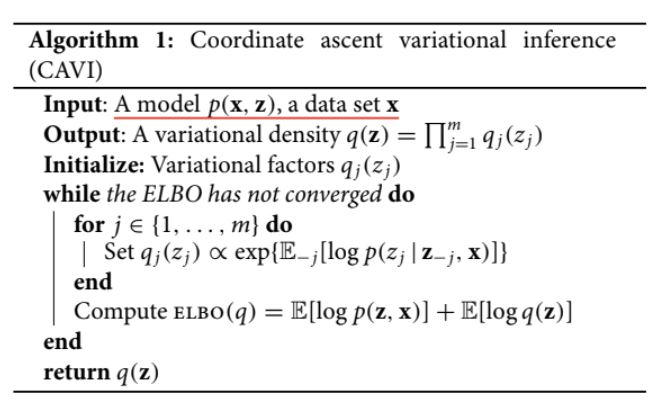
- In the update steps for CAVI, we can explicitly identify the form of the distribution of \(q_j(z_j)\) usually (e.g. binomial, poisson, normal, etc.) when we are working with exponential families and conditionally conjugate models. This makes the update steps easy, as we know the explicit update form of the variational parameters in each iteration.
CAVI worked example
- We apply CAVI to a simple mixture of Gaussians, with K mixture components and n real-valied data points \(x_{1:n}\). The latent variables are K real-valued mean parameters \(\boldsymbol{\mu}=\mu_{1:k}\) and n latent-class assignments \(\textbf{c}=c_{1:n}\), where \(c_i\) is an indicator (one-hot) K-vector.
- Derivations of the ELBO, and variational updates for the cluster assignment \(c_i\) and k-th mixture component \(\mu_k\) is shown here.
sessionInfo()R version 4.0.2 (2020-06-22)
Platform: x86_64-w64-mingw32/x64 (64-bit)
Running under: Windows 10 x64 (build 19041)
Matrix products: default
locale:
[1] LC_COLLATE=English_Australia.1252 LC_CTYPE=English_Australia.1252
[3] LC_MONETARY=English_Australia.1252 LC_NUMERIC=C
[5] LC_TIME=English_Australia.1252
system code page: 949
attached base packages:
[1] stats graphics grDevices utils datasets methods base
other attached packages:
[1] workflowr_1.6.2
loaded via a namespace (and not attached):
[1] Rcpp_1.0.5 rstudioapi_0.13 whisker_0.4 knitr_1.30
[5] magrittr_2.0.1 R6_2.5.0 rlang_0.4.10 stringr_1.4.0
[9] tools_4.0.2 xfun_0.20 git2r_0.27.1 htmltools_0.5.0
[13] ellipsis_0.3.1 rprojroot_2.0.2 yaml_2.2.1 digest_0.6.27
[17] tibble_3.0.4 lifecycle_0.2.0 crayon_1.3.4 later_1.1.0.1
[21] vctrs_0.3.6 promises_1.1.1 fs_1.5.0 glue_1.4.2
[25] evaluate_0.14 rmarkdown_2.6 stringi_1.5.3 compiler_4.0.2
[29] pillar_1.4.7 httpuv_1.5.4 pkgconfig_2.0.3